Minh Tran 52 Followers

(A) Delayed XOR task setup, shown after training. WebFor supervised learning problems, many performance metrics measure the amount of prediction error. \text{prediction/estimate:}\hspace{.6cm} \hat{y} &= \hat{f}(x_{new}) \nonumber \\ , has zero mean and variance Learn more about BMC . n

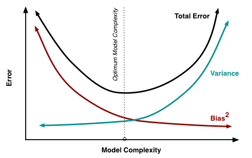
In machine learning, our goal is to find the sweet spot between bias and variance a balanced model thats neither too simple nor too complex.

(B) To formulate the supervised learning problem, these variables are aggregated in time to produce summary variables of the state of the network during the simulated window. The target Y is set to Y = 0.1. This linear dependence on the maximal voltage of the neuron may be approximated by plasticity that depends on calcium concentration; such implementation issues are considered in the discussion. Here we assume that T is sufficiently long for the network to have received an input, produced an output, and for feedback to have been distributed to the system (e.g. {\displaystyle \varepsilon }

Each model is created by using a sample of ( y) (, y) data. Importantly, neither activity of upstream neurons, which act as confounders, nor downstream non-linearities bias the results. In other words, test data may not agree as closely with training data, which would indicate imprecision and therefore inflated variance. If it does not work on the data for long enough, it will not find patterns and bias occurs. i {\displaystyle {\hat {f}}} Causal inference is, at least implicitly, the basis of reinforcement learning. The variance will increase as the model's complexity increases, while the bias will decrease. Maximum Likelihood Estimation 6. Figure 9: Importing modules. in the form of dopamine signaling a reward prediction error [25]). This suggests the SDE provides a more scale-able and robust estimator of causal effect for the purposes of learning in the presence of confounders. (D) Schematic showing how spiking discontinuity operates in network of neurons. Funding acquisition, In the following example, we will have a look at three different linear regression modelsleast-squares, ridge, and lassousing sklearn library.

We approximate this term with its mean: Citation: Lansdell BJ, Kording KP (2023) Neural spiking for causal inference and learning. {\displaystyle N_{1}(x),\dots ,N_{k}(x)} In this case there is a more striking difference between the spiking discontinuity and observed dependence estimators. Capacity, Overfitting and Underfitting 3. Further experiments with the impact of learning window size in other learning rules where a pseudo-derivative type approach to gradient-based learning is applied can be performed, to establish the broader relevance of the insights made here. That is, let Zi be the maximum integrated neural drive to the neuron over the trial period. These differences are called errors. Technically, we can define bias as the error between average model prediction and the ground truth. Visualization, n

x This proposal provides insights into a novel function of spiking that we explore in simple networks and learning tasks. Stock Market Import Export HR Recruitment, Personality Development Soft Skills Spoken English, MS Office Tally Customer Service Sales, Hardware Networking Cyber Security Hacking, Software Development Mobile App Testing, Download The asymptotic bias is directly related to the learning algorithm (independently of the quantity of data) while the overfitting term comes from the fact that the amount of data is limited. Methodology, This book is for managers, programmers, directors and anyone else who wants to learn machine learning.

to be minimal, both for

The observed dependence is biased by correlations between neuron 1 and 2changes in reward caused by neuron 1 are also attributed to neuron 2. https://doi.org/10.1371/journal.pcbi.1011005.g003. To show this we replace with a type of finite difference operator: x ( Dashed lines show the observed-dependence estimator, solid lines show the spiking discontinuity estimator, for correlated and uncorrelated (unconfounded) inputs, over a range of window sizes p. The observed dependence estimator is significantly biased with confounded inputs.



The same reward function is used as in the wide network simulations above, except here U is a vector of ones. For the deep network (Fig 5B), a two-hidden layer neural network was simulated.

The success of backpropagation suggests that efficient methods for computing gradients are needed for solving large-scale learning problems.

When an agent has limited information on its environment, the suboptimality of an RL algorithm can be decomposed into the sum of two terms: a term related to an asymptotic bias and a term due to overfitting. Plots show the causal effect of each of the first hidden layer neurons on the reward signal. In this section we discuss the concrete demands of such learning and how they relate to past experiments.

Softmax output above 0.5 indicates a network output of 1, and below 0.5 indicates 0. x WebBias-variance tradeo Inherent tradeoff between capturing regularities in the training data and generalizing to unseen examples. The term variance relates to how the model varies as different parts of the training data set are used. This balance is 1 In this paper SDE based learning was explored in the context of maximizing a reward function or minimizing a loss function. This shows that over a range of network sizes and confounding levels, a spiking discontinuity estimator is robust to confounding. The same simple model can be used to estimate the dependence of the quality of spike discontinuity estimates on network parameters. Example algorithms used for supervised and unsupervised problems. On one hand, we need flexible enough model to find \(f\) without imposing bias. underfit) in the data. Regularization methods introduce bias into the regression solution that can reduce variance considerably relative to the ordinary least squares (OLS) solution. We believe that focusing on causality is essential when thinking about the brain or, in fact, any system that interacts with the real world. We compare a network simulated with correlated inputs, and one with uncorrelated inputs. In the above equation, Y represents the value to be predicted. Within the field of machine learning, there are two main types of tasks: supervised, and unsupervised. This is the case in simulations explored here. where i, li and ri are the linear regression parameters. y ( Note that Si given no spike (the distribution on the RHS) is not necessarily zero, even if no spike occurs in that time period, because si(0), the filtered spiking dynamics at t = 0, is not necessarily equal to zero. Each layer had N = 10 neurons. The random variable Z is required to have the form defined above, a maximum of the integrated drive.

Reward-modulated STDP (R-STDP) can be shown to Answer: Supervised learning involves training a model on labeled data, where the Thus estimating the causal effect is similar to taking a finite difference approximation of the reward.

Computationally, despite a lot of recent progress [15], it remains challenging to create spiking neural networks that perform comparably to continuous artificial networks. This may be communicated by neuromodulation.
For instance, the LIF neural network implemented in Figs 24 has a fixed threshold. \(\text{nox} = f(\text{dis}, \text{zn})\), Machine Learning for Data Science (Lecture Notes). In a causal Bayesian network, the probability distribution is factored according to a graph, [27].

Machine learning models cannot be a black box. {\displaystyle x_{i}} Variance specifies the amount of variation that the estimate of the target function will change if different training data was used. y This reflects the fact that a zero-bias approach has poor generalisability to new situations, and also unreasonably presumes precise knowledge of the true state of the world. Bias & Variance of Machine Learning Models The bias of the model, intuitively speaking, can be defined as an affinity of the model to make predictions or estimates based on only certain features of the dataset. Bias: how closely does your model t the

To investigate the robustness of this estimator, we systematically vary the weights, wi, of the network. https://doi.org/10.1371/journal.pcbi.1011005.s003. Free, Enroll For

Bias is the difference between the average prediction and the correct value. Our approach is inspired by the regression discontinuity design commonly used in econometrics [34]. For inputs that place the neuron just below or just above its spiking threshold, the difference in the state of the rest of the network becomes negligible, the only difference is the fact that in one case the neuron spiked and in the other case the neuron did not. In Machine Learning, error is used to see how accurately our model can predict on data it uses to learn; as well as new, unseen data. From this a cost/reward function of R = |U s Y| is computed. Having understood how the causal effect of a neuron can be defined, and how it is relevant to learning, we now consider how to estimate it. Variance. However, if being adaptable, a complex model ^f f ^ tends to vary a lot from sample to sample, which means high variance. {\displaystyle P(x,y)} This is further skewed by false assumptions, noise, and outliers. We can implement this as a simple learning rule that illustrates how knowing the causal effect impacts learning. The network is presented with this input stimulus for a fixed period of T seconds. , A number of replacements have been explored: [44] uses a boxcar function, [47] uses the negative slope of the sigmoid function, [45] explores the so-called straight-through estimatorpretending the spike response function is the identity function, with a gradient of 1.

( For this we use the daily forecast data as shown below: Figure 8: Weather forecast data. Interested in Personalized Training with Job Assistance? These ideas have extensively been used to model learning in brains [1622]. The three terms represent: Since all three terms are non-negative, the irreducible error forms a lower bound on the expected error on unseen samples. The problem of coarse-graining, or aggregating, low-level variables to obtain a higher-level model amenable to causal modeling is a topic of active research [62, 63]. y That is, how does a neuron know its effect on downstream computation and rewards, and thus how it should change its synaptic weights to improve? Yet, despite these ideas, we may still wonder if there are computational benefits of spikes that balance the apparent disparity in the learning abilities of spiking and artificial networks.

The biasvariance dilemma or biasvariance problem is the conflict in trying to simultaneously minimize these two sources of error that prevent supervised learning algorithms Today, computer-based simulations are widely used in a range of industries and fields for various purposes. here. x Below we show how the causal effect of a neuron on reward can be defined and used to maximize this reward. Proximity to the diagonal line (black curve) shows these match. Curves show mean plus/minus standard deviation over 50 simulations. On the other hand, variance creates variance errors that lead to incorrect predictions seeing trends or data points that do not exist. No, Is the Subject Area "Learning" applicable to this article? First, a neuron assumes its effect on the expected reward can be written as a function of Zi which has a discontinuity at Zi = , such that, in the neighborhood of Zi = , the function can be approximated by either its 0-degree (piecewise constant version) or 1-degree Taylor expansion (piecewise linear). The discontinuity-based method provides a novel and plausible account of how neurons learn their causal effect. QQ-plot shows that Si following a spike is distributed as a translation of Si in windows with no spike, as assumed in (12). It turns out that the our accuracy on the training data is an upper bound on the accuracy we can expect to achieve on the testing data. Overall, corrected estimates based on spiking considerably improve on the naive implementation. The resulting heuristics are relatively simple, but produce better inferences in a wider variety of situations.[20].

[11] argue that the biasvariance dilemma implies that abilities such as generic object recognition cannot be learned from scratch, but require a certain degree of "hard wiring" that is later tuned by experience. If you are facing any difficulties with the new site, and want to access our old site, please go to https://archive.nptel.ac.in. There are four possible combinations of bias and variances, which are represented by the below diagram: Low-Bias, Low-Variance: The D Suppose that we have a training set consisting of a set of points It suggests that methods from causal inference may provide efficient algorithms to estimate reward gradients, and thus can be used to optimize reward. label) in the training data was plugged into the loss function, which governed the process of getting optimal model. Model validation methods such as cross-validation (statistics) can be used to tune models so as to optimize the trade-off. {\displaystyle D=\{(x_{1},y_{1})\dots ,(x_{n},y_{n})\}}

Thus R-STDP can be cast as performing a type of causal inference on a reward The most important aspect of spike discontinuity learning is the explicit focus on causality. One way of resolving the trade-off is to use mixture models and ensemble learning. Bias is a phenomenon that occurs in the machine learning model wherein an algorithm is used and it does not fit properly.

When a confounded network (correlated noisec = 0.5) is used the spike discontinuity learning exhibits similar performance, while learning based on the observed dependence sometimes fails to converge due to the bias in gradient estimate.

This feature of simple models results in high bias. This is used in the learning rule derived below. This just ensures that we capture the essential patterns in our model while ignoring the noise present it in. To remove confounding, spiking discontinuity learning considers only the marginal super- and sub-threshold periods of time to estimate . f There is always a tradeoff between how low you can get errors to be.

However, the aggregate variables do not fully summarize the state of the network throughout the simulation. However, once confounding is introduced, the error increases dramatically, varying over three orders of magnitude as a function of correlation coefficient. If drive is above the spiking threshold, then Hi is active.

Estimators, Bias and Variance 5.

Only for extremely high correlation values or networks with a layer of one thousand neurons does it fail to produce estimates that are not very well aligned with the true causal effects. Yes {\displaystyle {\text{MSE}}} ; In these simulations updates to are made when the neuron is close to threshold, while updates to wi are made for all time periods of length T. Learning exhibits trajectories that initially meander while the estimate of settles down (Fig 4C).

There are two main types of errors present in any machine learning model. The option to select many data points over a broad sample space is the ideal condition for any analysis. Therefore, increasing data is the preferred solution when it comes to dealing with high variance and high bias models. WebThis results in small bias. Taken together, this means the graph describes a causal Bayesian network over the distribution . thus noise in this layer is not correlated and any correlations between neural activity in the second layer come from correlated activity in the first layer. But, too flexible model will chase non-existing patterns in \(\varepsilon\) leading to unwanted variability. Determining the causal effect analytically is in general intractable. These choices were made since they showed better empirical performance than, e.g. Different choices of refractory period were not shown to affect SDE performance (S1 Fig). The spiking discontinuity approach requires that H is an indicator functional, simply indicating the occurrence of a spike or not within window T; it could instead be defined directly in terms of Z. Thus it is an approach that can be used in more neural circuits than just those with special circuitry for independent noise perturbations. This section shows how this idea can be made more precise.

f Bias in this context has nothing to do with data. WebBias. Here i, li and ri are nuisance parameters, and i is the causal effect of interest.
Of course, we cannot hope to do so perfectly, since the SDE works better when activity is fluctuation-driven and at a lower firing rate (Fig 3C). an SME, Resume (E) Model notation. We can see that as we get farther and farther away from the center, the error increases in our model.

In this article - Everything you need to know about Bias and Variance, we find out about the various errors that can be present in a machine learning model. There are, of course, pragmatic reasons for spiking: spiking may be more energy efficient [6, 7], spiking allows for reliable transmission over long distances [8], and spike timing codes may allow for more transmission bandwidth [9]. The fact that it does not communicate its continuous membrane potential is usually seen as a computational liability. Please let us know by emailing blogs@bmc.com. The standard definition of a causal Bayesian model imposes two constraints on the distribution , relating to: To use this theory, first, we describe a graph such that is compatible with the conditional independence requirement of the above definition. f ( severing the connection from xt to ht for all t renders H independent of X. Here we propose the spiking discontinuity is used by a neuron to efficiently estimate its causal effect. To test the ability of spiking discontinuity learning to estimate causal effects in deep networks, the learning rule is used to estimate causal effects of neurons in the first layer on the reward function R. https://doi.org/10.1371/journal.pcbi.1011005.s001. Thus if the noise a neuron uses for learning is correlated with other neurons then it can not know which neurons changes in output is responsible for changes in reward. > For instance, there is some evidence that the relative balance between adrenergic and M1 muscarinic agonists alters both the sign and magnitude of STDP in layer II/III visual cortical neurons [59]. We present the first model to propose a neuron does causal inference. The model's simplifying assumptions simplify the target function, making it easier to estimate. If this is the case, our model cannot perform on new data and cannot be sent into production., This instance, where the model cannot find patterns in our training set and hence fails for both seen and unseen data, is called Underfitting., The below figure shows an example of Underfitting. {\displaystyle f_{a,b}(x)=a\sin(bx)} a web browser that supports

contain noise

(A) Estimates of causal effect (black line) using a constant spiking discontinuity model (difference in mean reward when neuron is within a window p of threshold) reveals confounding for high p values and highly correlated activity. A lot of recurrent neural networks, when applied to spiking neural networks, have to deal with propagating gradients through the discontinuous spiking function [5, 4448]. Statistically, within a small interval around the threshold spiking becomes as good as random [2830]. , we show that. This means inputs that place a neuron close to threshold, but do not elicit a spike, still result in plasticity. Yet machine learning mostly uses artificial neural networks with continuous activities. In this way the spiking discontinuity may allow neurons to estimate their causal effect. Such an interpretation is interestingly in line with recently proposed ideas on inter-neuron learning, e.g., Gershman 2023 [61], who proposes an interaction of intra-cellular variables and synaptic learning rules can provide a substrate for memory. WebUnsupervised Learning Convolutional Neural Networks (CNN) are a type of deep learning architecture specifically designed for processing grid-like data, such as images or time-series data. x

The goal of any supervised machine learning has only two parameters ( Reward-modulated STDP (R-STDP) can be shown to approximate the reinforcement learning policy gradient type algorithms described above [50, 51].

Any issues in the algorithm or polluted data set can negatively impact the ML model.

From this setup, each neuron can estimate its effect on the function R using either the spiking discontinuity learning or the observed dependence estimator. Further, for spiking discontinuity learning, plasticity should be confined to cases where a neurons membrane potential is close to threshold, regardless of spiking. ) The adaptive LIF neurons do have a threshold that adapts, based on recent spiking activity. Selecting the correct/optimum value of will give you a balanced result.



Balanced Bias And Variance In the model. Ten simulations were run for each value of N and c in Fig 5A. STDP performs unsupervised learning, so is not directly related to the type of optimization considered here.

x Learning by operant conditioning relies on learning a causal relationship (compared to classical conditioning, which only relies on learning a correlation) [27, 3537]. Alignment between the true causal effects and the estimated effects is the angle between these two vectors. then that allows it to estimate its causal effect. There are two factors that cast doubt on the use of reinforcement learning-type algorithms broadly in neural circuits. p = 1 represents the observed dependence, revealing the extent of confounding (dashed lines). } Of course, given our simulations are based on a simplified model, it makes sense to ask what neuro-physiological features may allow spiking discontinuity learning in more realistic learning circuits. Here is a set of nodes that satisfy the back-door criterion [27] with respect to Hi R. By satisfying the backdoor criterion we can relate the interventional distribution to the observational distribution. No, Is the Subject Area "Network analysis" applicable to this article?

x When applied to the toy LIF network, the online learning rule (Fig 4A) estimates over the course of seconds (Fig 4B).

Because of the fact that the aggregated variables maintain the same ordering as the underlying dynamic variables, there is a well-defined sense in which R is indeed an effect of Hi, not the other way around, and therefore that the causal effect i is a sensible, and not necessarily zero, quantity (Fig 1C and 1D). The latter is known as a models generalisation performance. To mitigate how much information is used from neighboring observations, a model can be smoothed via explicit regularization, such as shrinkage. x However, complexity will make the model "move" more to capture the data points, and hence its variance will be larger. ) We will be using the Iris data dataset included in mlxtend as the base data set and carry out the bias_variance_decomp using two algorithms: Decision Tree and Bagging. Such perturbations come at a cost, since the noise can degrade performance. {\displaystyle f(x)}

Precision is a description of variance and generally can only be improved by selecting information from a comparatively larger space. We start with very basic stats and algebra and build upon that. Its a delicate balance between these bias and variance. This works because the discontinuity in the neurons response induces a detectable difference in outcome for only a negligible difference between sampled populations (sub- and super-threshold periods). We show that this idea suggests learning rules that allows a network of neurons to learn to maximize reward, particularly in the presence of confounded inputs. , Definition 1.

It turns out that whichever function ,

Emory Crna Application, Pi Kappa Phi Secrets Revealed, Articles B